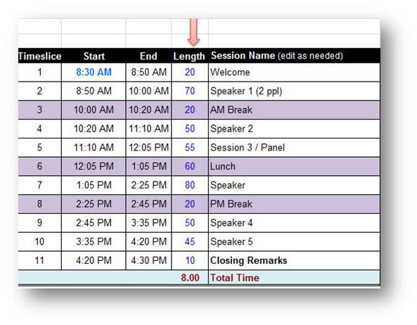
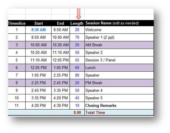
As part of RedCape’s webinar series “How’d They Do That?” here is an example Excel tool that allows you to enter length (in minutes) when creating a meeting schedule to automatically calculate the start and end times for each speaker or topic, plus breaks. This is a great tool! Now let’s see how they did that. [Here’s our final version: http://sdrv.ms/OEutz7]

Overall steps:

1. Create a new Excel file and set up the table
2. Create the calculation for end times
3. Fill in the start times
4. Insert the session lengths
5. Format the table
6. (Bonus) Add conditional formatting for breaks & lunch

Step by Step instructions

These are the step by step instructions using Excel 2010, but can be used in any version of Excel (PC or Mac).

Step 1 – Create a new Excel file and set up the table

1. Launch Excel to create a new workbook.
2. In cell B4 type Timeslice and hit [Tab]
   (note: you can change the column name if you prefer)
3. In cell C4 type Start and hit [Tab]
4. In cell D4 type End and hit [Tab]
5. In cell E4 type Length and hit [Tab]
6. In cell F4 type Session Name and hit [Enter], which brings the active cell to B5
7. In cell B5 type 1 and hit [Enter]
8. In cell B6 type 2 and hit [Enter]
9. Select both B5 and B6 and use autofill to fill the series to 11. (How to: Fill a series of numbers, dates, or other built-in series items)
10. In cell C5, type the start time 8:30 AM and hit [Tab] twice so that your active cell is E5.
11. In cell E5, type 20 and hit [Tab].
12. In cell F5, type Welcome and hit [Enter].
13. Select cell B4 (or any cell with data in it) and on the Home tab, in the Styles group, click Format as a Table and choose the very first option “Table Style Light 1″. Make sure “My table has headers” is checked and click Ok.

Step 2 – Create the calculation for end times

We are going to use the Time() function to add minutes. The Time() function allows us to specify hours, minutes, and seconds. Because we are working with minutes, we will use 0 for the hours, the Length column for the minutes, and 0 for the seconds.

1. In cell D5, type an equal sign (=) and then point to cell C5, which is the Start Time for row 5.

2. Type a plus sign (+) for adding.

3. Then begin typing Time(, which displays the autocomplete tip for the Time function.

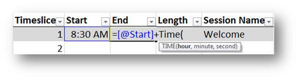
4. Type 0 for the hours since we are only focused on minutes and then type a comma (,) to move to the minutes.

5. Type [Length] to use the value in the Length column and then type a comma (,) to move to the seconds.

6. Type 0) for seconds since we are only focused on minutes. Then hit [Tab].

Note: The function should look like this: =[@Start]+TIME(0,[Length],0)

7. Note: if you get number signs (######) in the cells it means that your column isn’t wide enough. Change the width of column D to see the End Times. Tip: Position the mouse pointer between column headers D and E so that your mouse turns into a double-headed arrow. Double-click and you should get the best fit for that column.

8. This is what your table should look like at this point. We haven’t filled in the Start times or the Length of the remaining session names.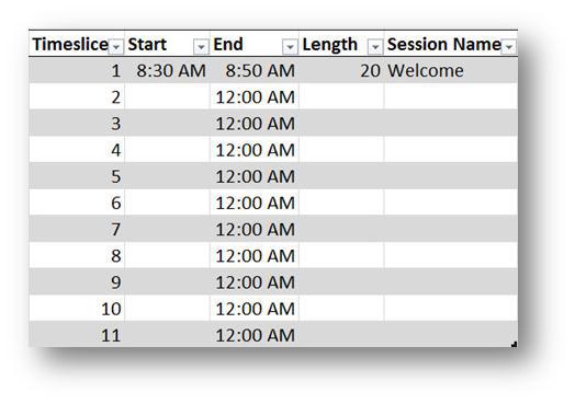

Step 3 – Fill in the start times

The only start time you need is the very first one. Once the end time is calculated for each row, that end time can be used as the start time for the next row.

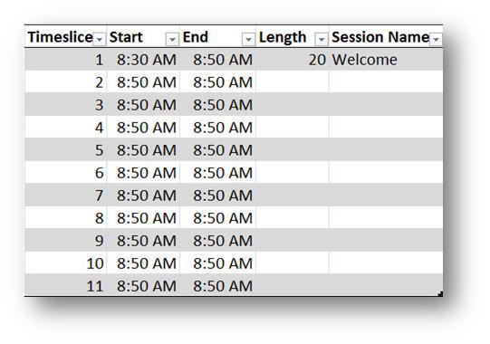
1. In cell C6, type an equal sign (=) and then click on cell D5, which is the end time for the previous line. Then hit [Enter].
2. Copy that calculation to the remaining Start time rows that are empty by using Autofill. Select C6 and position your mouse on the bottom right hand corner of the cell so that your mouse turns into a little black plus sign. Drag (using the black plus sign) down to the last row so that your table now looks like this:

Step 4 – Insert the session lengths

Now we’re ready to use our table to calculate the start and end times for our meeting.

1. Because we know what the structure of our meeting is, let’s first type our Session Names. Start in cell F6 and type the following:
   1. Speaker 1 and hit [Enter].
   2. AM Break [Enter]
   3. Speaker 2 [Enter]
   4. Panel [Enter]
   5. Lunch [Enter]
   6. Speaker 3 [Enter]
   7. PM Break [Enter]
   8. Speaker 4 [Enter]
   9. Speaker 5 [Enter]
   10. Closing Remarks [Enter]
2. Enter the times for each Session Name. Start in cell E6 for Speaker 1 and type the following:
   1. Type 70 and hit [Enter]
      Note: if you get number signs (######) in the cells it means that your column isn’t wide enough. Change the width of column C to see the Start Times. Tip: Position the mouse pointer between column headers C and D so that your mouse turns into a double-headed arrow. Double-click and you should get the best fit for that column.
   2. In cell E7 for the AM Break, type 20 and then hit [Enter]
   3. Fill in the times as seen in this example:

Step 4 – Format the table

There are a few things we can do to the table to make it look even better!

1. Let’s center align the Timeslice and Length columns. Hover your mouse over the Timeslice header (a little bit above the word “Timeslice”) until you see a black arrow point down. Once you see the black arrow, click once to select the column in that table. Then apply center alignment. Repeat for the Length column.
2. Add the total row
   1. Click anywhere in your table so that you see the Table Tools Design tab on your Ribbon. Click on the Design tab to activate the ribbon and view the table commands.
   2. In the Table Style Options group, click Total Row.
   3. In cell E16, type the following formula to calculate the total hours: =sum([Length])/60
   4. Format the total hours to include 2 decimals places: Select cell E16 and on the Home tab, in the Number group, click Increase Decimal twice.
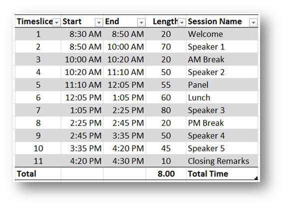
   5. In cell F16, type Total Time. Your Table should look like this:

   

3. Style your table using one of the Built-in table styles
   1. Click in your table to display the Table Tools Design Tab ribbon. Click on the Design tab to activate the ribbon if it isn’t already showing.
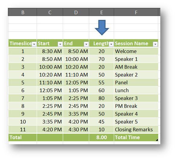
   2. In the Table Styles group, explore the built-in table styles and select your preferred one. I used “Table Styles Medium 11″, which is green.
4. Let’s add a groovy arrow that points to the Length column so that when we use the tool in the future, we’ll know that we only have to update the Length column.
   1. On the Insert tab, in the Illustrations group, click the Shapes drop down.
   2. In the Block Arrows category, choose a block arrow pointing down.
   3. Draw the arrow above the Length column.
   4. (optional) use the Drawing Tools ribbon to format your new arrow (perhaps change the arrow using one of the many built-in Shape Styles).
   5. (optional) add another arrow pointing down at the Session Name column, which is another column you will modify.
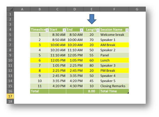
   6. This is what the table looks like now (I did not do the optional steps d and e above):

Step 5 – BONUS STEP – Add conditional formatting to highlight rows for breaks & lunch

In our original example, the rows for AM / PM Breaks, as well as lunches, are highlighted grey. Rather than manually highlight those rows, let’s use conditional formatting to highlight any row where we have a break or lunch. This will save us a lot of time later when we’re drafting the schedule so that if we decide to move the breaks or lunch in the schedule, we won’t have to worry about removing the shading.

8/31/12 Blog Update: Thanks to Seth Hart at the Texas Workforce Commission who submitted a more efficient method for setting up conditional formatting for breaks. See below step #4 for details.

1. Select cells B5 throughF15.
2. On the Home tab, in the Styles group, click Conditional Formatting and select New Rule…
3. From the Select a Rule Type section, select Use a formula
4. to determine which cells to format.
5. Under Format values where this formula is true, type =$F5=”AM Break” (with the quotes)
6. Click the Format button to launch the Format Cells dialog box.
7. Click the Fill tab and choose the bright yellow color from the color palette.
8. Click Ok to close the Format Cells dialog box.
9. Click Ok to close Conditional Formatting. Row 3 should now be highlighted yellow like this:

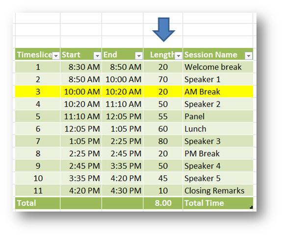
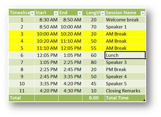
10. To test the conditional formatting, change a couple of the Session Names to AM Breakand the other rows should highlight as seen in the screenshot below.IMPORTANT: Be sure to change them back to their original Session Names and proceed to the next steps to create the remaining conditional formats for PM Break, Lunch and one for Break, just in case you use just the word “Break”.

1. Select cells B5 throughF15.
2. On the Home tab, in the Styles group, click Conditional Formatting and select New Rule…
3. From the Select a Rule Type section, select Use a formula to determine which cells to format.
4. Under Format values where this formula is true, type =$F5=”PM Break” (with the quotes)
5. Click the Format button to launch the Format Cells dialog box.
6. Click the Fill tab and choose the bright yellow color from the color palette.
7. Click Ok to close the Format Cells dialog box.
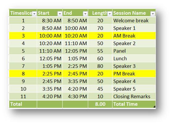
8. Click Ok to close Conditional Formatting. Row 8 should now be highlighted yellow like this:

1. Select cells B5 throughF15.
2. On the Home tab, in the Styles group, click Conditional Formatting and select New Rule…
3. From the Select a Rule Type section, select Use a formula to determine which cells to format.
4. Under Format values where this formula is true, type =$F5=”Lunch” (with the quotes)
5. Click the Format button to launch the Format Cells dialog box.
6. Click the Fill tab and choose the bright yellow color from the color palette.
7. Click Ok to close the Format Cells dialog box.
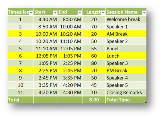
8. Click Ok to close Conditional Formatting. Row 8 should now be highlighted yellow like this:

4. (Optional) Create a yellow highlight for the rows if the Session Name = “Break”
The conditional formatting will only work if you use the exact terms AM Break, PM Break or Lunch. What if you type “Break” as the session name? Try this on your own! Create a new conditional format so that the row gets highlighted yellow if the Session Name is “Break”.

8/31/12 Blog Update – Here are the instructions on how to find any instance of the word “Break” in the Session Name and apply conditional formatting. This will eliminate the need to create three individual rules for AM Break, PM Break, and Break. Anytime the word “break” is in the name, let’s apply conditional formatting.

The rule is: =IsNumber(Search(“break”,$F5))

The Search() function returns a number value representing the character position of the word “break”. If it doesn’t find it, then it returns #Value, which is NOT a number. The IsNumber() function then returns the true or false value that we need to apply the conditional format. Brilliant!

We had lots of submissions during our webinar. Thank you to Seth Hart at the Texas Workforce Commission for submitting this one. Readers: if you have another suggestion, please leave a comment below. I’d love to see what else is out there.

Optional Step – Remove Gridlines

Whenever I create calculated tools like this, I like to remove the gridlines in the background. To do this, on the View tab, in the Show group, click Gridlines to deselect it.

This is what my final schedule looks like and here is the link to my final version: http://sdrv.ms/OEutz7. You are more than welcome to use it for your next meeting.

Submit your comments

Have a question or an idea on how to make the steps above even easier? Submit your feedback below.

Also, if you have a Microsoft Office tool or template that you would like us to feature in our How’d They Do That series, send your request to me at vsevans at redcapeco dot com.

Thanks for reading!! Until next time…